Evapotranspiration from Weather and Satellites

A complete guide to surface energy balance and crop-coefficient evapotranspiration in R with the sebkc package

This manual teaches the sebkc R package from the ground up. It assumes only basic R literacy and a first acquaintance with evapotranspiration (ET), and explains every term as it appears. Part 1 estimates ET from weather data — FAO-56 reference ET and the single/dual crop-coefficient water balance — needing nothing but numbers. Part 2 estimates ET from satellite imagery — the surface-energy-balance models (SEBAL, METRIC, SEBS, SEBI, SSEB, S-SEBI and the two-source TSEB) — on the bundled Landsat scene. Part 3 is a reference, a reproducibility script, a glossary and exercises, and Part 4 a set of student projects.

New — a plain-language companion. If your goal is simply “how much water does my crop need and how much must I irrigate?”, start with the practical companion guide, “How Much Water Does My Crop Need?” (crop_water_needs.html), which walks through real crop-water-needs assessments for farms near Kumasi with no jargon. This manual is the full technical reference behind it.

Dr George Owusu Department of Geography and Resource Development, University of Ghana

Version 1.0-7
Package: sebkc
Core is pure R; spatial input uses 'raster' and 'sp'
For: hydrologists, agronomists, irrigation engineers, remote-sensing scientists
     and anyone estimating evapotranspiration from weather or satellite data
Prerequisites: basic R literacy
License: GPL-2

Every number and figure in this manual was produced by running the package. The script that regenerates them, reproduce_manual.R, ships in this folder; its console output is repro_output.txt and its figures are in figures/. Run it and you get exactly the tables and plots printed here. (The numbers were produced on R 4.6.0 with sebkc 1.0-7.)

Part 1 — ET from weather data (point) 1. What this package does 2. Installing and loading 3. Two ways in: point vs satellite 4. ETo: 24-hour reference ET (FAO-56) 5. ETohr: hourly reference ET 6. weather: retrieving weather data 7. kc: single and dual crop coefficients, and the water balance 8. cal.kc: calibrating the water balance 9. biomass: crop yield from temperature and radiation

Part 2 — ET from satellite imagery (spatial) 10. From image to ET: the surface energy balance 11. sebkcstack and landsat578: from raw bands to albedo, NDVI and Ts 12. coldTs / hotTs: the anchor pixels 13. sebal: SEBAL and METRIC 14. The one-source family: sebs, sebi, sseb, ssebi 15. tseb: the two-source model 16. Comparing the models 17. wdi: the water deficit index 18. Coupling evaporative fraction to the FAO-56 water balance

Part 3 — reference 19. Function and argument reference 20. The bundled data 21. Reproducing the figures 22. Glossary 23. Exercises

Part 4 — projects 24. The project brief template 25. Agriculture and irrigation projects 26. Hydrology and water-resources projects 27. Remote-sensing and land-surface projects 28. Climate and environment projects 29. Methods project

How to cite this manual References

PART 1 — ET from weather data (point)

1. What this package does

Evapotranspiration (ET) — the water that leaves the land as evaporation from soil and transpiration from plants — is the largest consumer of irrigation water and a central term in every water balance. sebkc estimates it two complementary ways, and integrates the two:

From weather data (Part 1). The FAO-56 method computes a reference ET (ETo) for a standard grass surface, then scales it by a crop coefficient (kc) to a specific crop, inside a day-by-day soil-water balance that tracks soil moisture, irrigation need and crop stress. Nothing but weather numbers is required.
From satellite imagery (Part 2). The surface energy balance partitions the net radiation a pixel absorbs into heating the air, heating the soil, and evaporating water; the last term is ET. sebkc implements the major one-source models (SEBAL, METRIC, SEBS, SEBI, SSEB, S-SEBI) and the two-source TSEB, turning a Landsat scene into a map of ET.
The integration. The satellite evaporative fraction can be fed straight into the FAO-56 water balance (kc), so a map of remotely sensed ET becomes a spatial irrigation-scheduling model. That coupling is the package’s distinctive contribution.

The problem this manual follows — irrigation water in Kumasi. The bundled data are a Landsat scene over Kumasi, Ghana, plus a short irrigation record. We ask: how much water does the reference crop demand (Part 1), how much is the land actually evapotranspiring pixel by pixel (Part 2), and how do the two combine into an irrigation schedule (Section 18)? Every function is demonstrated on that thread.

Key terms, defined once

Reference ET (ETo) — ET of a standard, well-watered grass; the climatic demand, in mm/day.
Crop coefficient (Kc) — the ratio of a crop’s ET to reference ET; ETc = Kc · ETo.
Net radiation (Rn) — energy absorbed by the surface [W/m²].
Sensible heat (H) — energy heating the air; soil heat (G) — energy heating the ground; latent heat (LE) — energy evaporating water. The surface energy balance is Rn = G + H + LE.
Evaporative fraction (EF) — the share of available energy going to ET, EF = LE / (Rn − G); the bridge between the satellite models and daily ET.

2. Installing and loading

From CRAN (recommended — dependencies are handled automatically):

install.packages("sebkc")
library(sebkc)

Or the development version from GitHub:

# install.packages("remotes")
remotes::install_github("gowusu/sebkc")

The spatial workflow (Part 2) uses raster and sp, which install with the package. System note. Verified on R 4.6.0 (Windows) with raster 3.6-32 and sp 2.2-3.

3. Two ways in: point vs satellite

sebkc has two families of functions that meet in the middle:

Table 1: The two ET pathways in sebkc and where they meet.

Pathway	Input	Functions	Output
Point (Part 1)	weather numbers	`ETo`, `ETohr`, `weather`, `kc`, `cal.kc`, `biomass`	reference/crop ET, water balance, yield
Satellite (Part 2)	Landsat / MODIS rasters	`landsat578`, `coldTs`/`hotTs`, `sebal`, `sebs`, `sebi`, `sseb`, `ssebi`, `tseb`, `wdi`	maps of Rn, H, G, LE, EF, ET
The bridge	satellite EF → FAO-56	`kc(kc = EF, ...)`	spatial water balance / irrigation need

Part 1 needs no imagery and runs instantly; start there.

4. `ETo`: 24-hour reference ET (FAO-56)

ETo() computes the daily reference evapotranspiration by the FAO-56 Penman–Monteith equation. With a full set of weather it reproduces the FAO textbook; with only Tmax and Tmin it falls back to the Hargreaves radiation estimate, so it always returns a number.

# minimal data (a warm, humid tropical day)
PET <- ETo(Tmax = 31, Tmin = 28, latitude = 5.6, DOY = "6-2-2001")
PET$ETo
#> 2.373                       # mm/day

# full data — FAO-56 Example 18, Brussels, 6 July
PET24 <- ETo(Tmax = 21.5, Tmin = 12.3, z = 10, uz = 2.78, altitude = 100,
             RHmax = 84, RHmin = 63, n = 9.25, DOY = 187, latitude = 50.8)
PET24$ETo
#> 3.88                        # mm/day — the FAO textbook value is 3.9

The full call reproduces ETo = 3.88 mm/day against the textbook’s 3.9, and returns the intermediate quantities too: net radiation Rn = 13.28 MJ/m²/day, the slope of the saturation-vapour-pressure curve = 0.1221 kPa/°C, the psychrometric constant y = 0.0666 kPa/°C, and the vapour-pressure deficit vpd = 0.589 kPa.

The FAO-56 Penman–Monteith equation (Allen et al., 1998, Eq. 6). Reference ET combines an energy term (net radiation) and an aerodynamic term (wind × vapour deficit):

$ET_o = \frac{0.408\,\Delta\,(R_n - G) + \gamma\,\dfrac{900}{T+273}\,u_2\,(e_s - e_a)}{\Delta + \gamma\,(1 + 0.34\,u_2)}$

where $\Delta$ is the slope of the saturation-vapour-pressure curve (slope), $\gamma$ the psychrometric constant (y), $u_2$ the 2-m wind speed, and $(e_s-e_a)$ the vapour-pressure deficit (vpd). When wind, humidity or sunshine are missing, sebkc estimates $R_n$ from temperature via the Hargreaves coefficient Krs (0.16 interior, 0.19 coastal).

Two arguments matter for later coupling: EF= accepts a satellite evaporative fraction and returns actual ET (ETa); Kc= accepts a crop coefficient and returns crop ET (ETc). surface= switches the reference between "grass" (default) and "alfalfa".

5. `ETohr`: hourly reference ET

For sub-daily work — matching a satellite overpass, say — ETohr() computes ET for a period of t1 hours centred on time, using mean temperature and humidity:

ET1 <- ETohr(Tmean = 38, RH = 52, DOY = 274, Lz = 15, t1 = 1, time = 14.5,
             Lm = 16.25, latitude = 16.22, uz = 3.3, Rs = 2.450)
ET1$ETo
#> 0.656                       # mm/hour

Lz and Lm are the longitudes of the time-zone centre and the site (both degrees west, positive), needed for the solar-time correction. The instantaneous ET at an overpass is what upscales, via the evaporative fraction, to a daily map in Part 2.

6. `weather`: retrieving weather data

weather() builds the ETo/kc inputs for a site from the NASA POWER daily data service (an internet connection is required). Give it a longitude/latitude and a date range; it returns temperature, humidity, wind, solar radiation and precipitation, already named and unit-ready for FAO-56:

kumasi <- weather(longitude = -1.5, latitude = 6.7,
                  NASA.SSE = list(from = "2001-04-01", to = "2001-04-07"))
d <- kumasi$NASA.SEE$data
d[, c("date","Tmax","Tmin","RH","uz","Rs","P")]
#>         date  Tmax  Tmin    RH   uz    Rs    P
#> 1 2001-04-01 34.01 23.84 74.99 2.50 22.41 6.73
#> 2 2001-04-02 33.33 23.39 77.89 2.91 22.63 5.28
#> 3 2001-04-03 30.30 23.47 81.28 3.01 10.49 4.27
#> ... (7 days)

The columns carry FAO-56 names and units: Tmax/Tmin/Tmean (°C), RH (%), uz (2-m wind, m/s), Rs (solar radiation, MJ/m²/day), P (mm/day) and altitude (m, from the POWER header), plus a calendar date and a numeric DOY. They feed ETo directly — row 1 above gives ETo = 5.32 mm/day. (An older station path, by WMO/airport code, is retained but its Weather Underground source was discontinued; use the coordinate/POWER path above.)

From download to ET. Because the columns are already FAO-56-ready, generating reference ET for every day is one sapply over the rows — and the precipitation P that POWER returns drives the water balance too:

d$ETo <- sapply(seq_len(nrow(d)), function(i)
  ETo(Tmax = d$Tmax[i], Tmin = d$Tmin[i], RHmax = d$RH[i], RHmin = d$RH[i],
      uz = d$uz[i], Rs = d$Rs[i], altitude = d$altitude[i],
      latitude = 6.7, DOY = d$date[i])$ETo)
round(d[, c("date","Tmax","Tmin","Rs","P","ETo")], 2)
#>         date  Tmax  Tmin    Rs    P  ETo
#> 1 2001-04-01 34.01 23.84 22.41 6.73 5.32
#> 2 2001-04-02 33.33 23.39 22.63 5.28 5.21
#> 3 2001-04-03 30.30 23.47 10.49 4.27 3.04   # cloudy day: low Rs -> low ETo
#> ...                                        # 10 days: mean ETo 4.59, total rain 30.3 mm

# feed the same POWER ETo and precipitation into the FAO-56 water balance
m <- kc(ETo = d$ETo, P = d$P, RHmin = 55, soil = "sandy loam", crop = "Broccoli", I = 0)
round(m$output[, c("Day","ETo","ETc","P","Drend")], 2)
#>    Day  ETo  ETc    P Drend
#> 1    1 5.32 4.70 6.73  0.67
#> ...
#> 10   10 4.50 1.74 1.03  8.32   # ~8 mm cumulative irrigation need after 10 rain-fed days

A few lines take you from a coordinate to a daily ET series and an irrigation-need estimate (Drend), entirely from real, downloaded weather — precipitation included.

Getting the data manually — no R needed. The same series is available from the web: - NASA POWER Data Access Viewer (point-and-click download): https://power.larc.nasa.gov/data-access-viewer/ - POWER API documentation (the endpoint weather() calls): https://power.larc.nasa.gov/docs/services/api/temporal/daily/ - POWER home: https://power.larc.nasa.gov

Other free weather/solar sources you can feed to ETo/kc: - Open-Meteo — historical + forecast API, no key: https://open-meteo.com - Copernicus ERA5 (CDS): https://cds.climate.copernicus.eu - NOAA Climate Data Online (GHCN stations): https://www.ncei.noaa.gov/cdo-web/ - a local met agency (e.g. the Ghana Meteorological Agency) for station records.

POWER covers ~1981 to near-present at ~0.5° resolution; for field-scale work a nearby ground station is preferable where available. This section needs a live connection and is not part of the offline reproduction.

7. `kc`: single and dual crop coefficients, and the water balance

kc() is the heart of Part 1. It turns reference ET into crop ET and runs a day-by-day FAO-56 soil-water balance — tracking depletion, irrigation need, runoff, deep percolation and crop stress. It has a backend of the FAO-56 tables, so naming a crop and soil is often enough.

The single vs dual coefficient. A single Kc lumps evaporation and transpiration into one curve; the dual Kc splits them into a basal transpiration coefficient Kcb and a soil-evaporation coefficient Ke, which is more accurate when the surface wets and dries between irrigations.

Crop ET and the dual coefficient (FAO-56). Crop ET scales reference ET by the crop coefficient, and the dual form splits that coefficient in two:

$ET_c = K_c\,ET_o, \qquad K_c = K_{cb}\,K_s + K_e$

where $K_{cb}$ is the basal (transpiration) coefficient, $K_e$ the soil-evaporation coefficient, and $K_s\in[0,1]$ a water-stress coefficient that drops below 1 when root-zone depletion exceeds the readily available water.

Reproducing the FAO-56 textbook. The package matches the worked examples:

# Example 32 — Broccoli, dual Kc, sprinkler irrigation
Ex32 <- kc(ETo = 7, P = 0, RHmin = 20, soil = "sandy loam", crop = "Broccoli",
           I = 10, kctype = "dual", u2 = 3, kc = c(0.9, 0, 0), h = 1, Zr = 0.1)
Ex32$output$fc        #> 0.526    fraction of ground covered
Ex32$output$Kc_adj    #> 1.301    adjusted crop coefficient

Switching the wetting method reproduces Examples 33 (furrow, fw = 0.3) and 34 (drip, fw = "drip"), giving Kc_adj = 0.66 and 0.651 respectively — lower, because wetting less of the surface leaves less to evaporate.

A multi-day water balance. The bundled irrigation.txt holds a 12-day record. Feeding its ETo, precipitation and irrigation columns runs the balance:

d <- read.table(system.file("extdata","sys","irrigation.txt", package = "sebkc"),
                header = TRUE)
m <- kc(ETo = d$ETo, P = d$P, RHmin = 35, soil = "sandy loam",
        crop = "Broccoli", I = d$I)
m$output[c("Day","ETo","Kc","ETc","TAW","RAW","AW_modelled","Runoff")]

Table 2: The FAO-56 water balance over 12 days (single-Kc, bundled irrigation data).

Day	ETo	Kc	ETc	TAW	RAW	AW_modelled
1	4.5	0.15	5.46	5	2.25	5.00
2	5.0	0.15	6.07	10	4.31	10.00
3	3.9	0.15	3.55	15	6.11	8.93
6	2.7	0.15	2.43	30	17.56	22.49
9	4.7	0.15	1.01	45	26.37	29.58
12	6.4	0.15	7.79	60	35.44	60.00

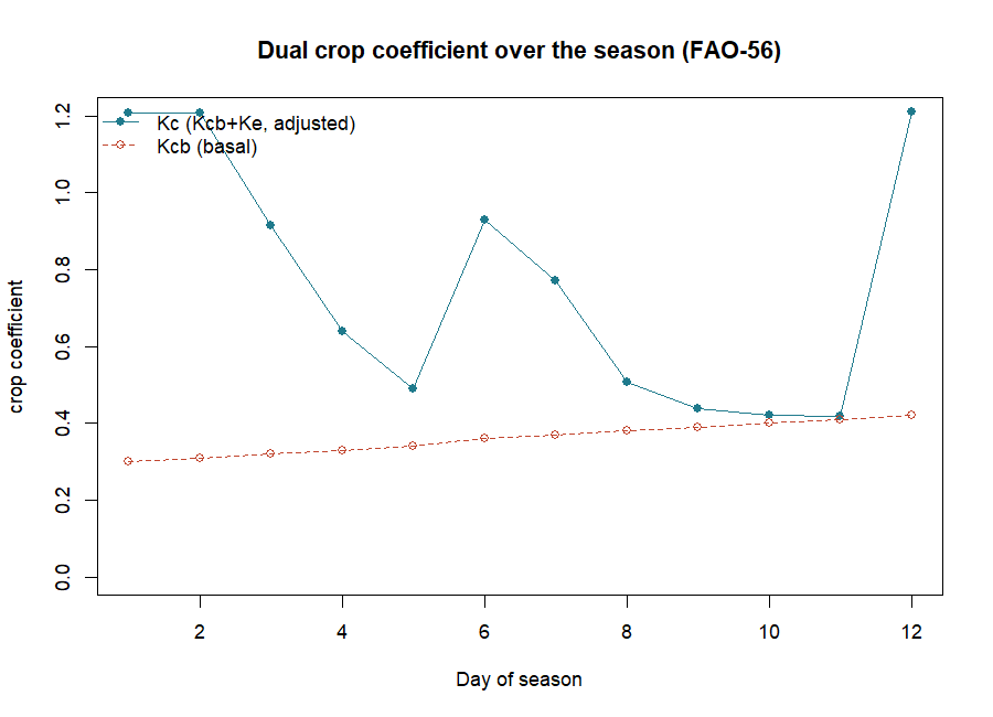
TAW is the total available water the root zone can hold, RAW the readily available part before stress begins, and AW_modelled the modelled soil water on the day. The output data frame carries ~40 columns in all — Ks, Kcb, Ke, Drend (the irrigation depth needed to refill the root zone), DP (deep percolation), CN (curve number) and more (Section 19). Running the dual model over the same days, with the bundled Kcb column and stage lengths, gives the classic season curve (Figure 1): the adjusted Kc (transpiration + evaporation spikes after wetting) rides above the smooth basal Kcb.

Figure 1: Dual crop coefficient over the season. The basal Kcb (dashed) is the transpiration curve; the adjusted Kc (solid) adds soil-evaporation spikes after each wetting, and dips where water stress reduces it. Kc_adj ranges 0.42–1.21, Kcb 0.30–0.42.

8. `cal.kc`: calibrating the water balance

Many of the balance’s parameters — field capacity FC, wilting point WP, curve number CNII, rooting depth Zr, the depletion fraction p, readily evaporable water REW — are rarely known exactly. cal.kc() calibrates them against measured soil-moisture observations by searching for the values that best reproduce the record. Supply the same call as kc() plus a column of measured soil water, and it returns the fitted parameters and goodness-of-fit. Use it whenever you have field measurements to anchor the model before trusting its irrigation recommendations. (Like weather, cal.kc needs user-supplied field data, so it is described here but not part of the offline reproduction — the only two functions in that category.)

9. `biomass`: crop yield from temperature and radiation

biomass() estimates crop biomass and yield from average temperature, shortwave radiation and the growing-season dates, using the FAO agro-ecological-zone method and a harvest index:

bm <- biomass(Tday = 26.9, T24 = 25.3, Rs = 452, latitude = 11.18, HI = 0.4,
              plantdate = "2015-05-1", harvestdate = "2015-08-29",
              adaptability = 3, LAI = 5, crop = "maize")
bm$yield
#> 9.822809                    # t/ha, maize, 120-day season

Passing vectors of latitude/Rs/Tday estimates several locations at once. Yield closes the loop from water (ET) to production — the quantity irrigation ultimately serves.

PART 2 — ET from satellite imagery (spatial)

Reading Part 2. Part 2 estimates actual ET pixel by pixel from a satellite image, where Part 1 estimated the crop’s demand from weather. The two meet in Section 18. The five terms you need: Rn (net radiation absorbed), G (soil heat), H (sensible heat warming the air), LE (latent heat = ET), and EF (evaporative fraction, the share of energy going to ET). Everything below is a different way of solving one equation for LE.

10. From image to ET: the surface energy balance

A satellite cannot see ET directly. What it sees — reflected sunlight (albedo), vegetation greenness (NDVI) and thermal emission (surface temperature Ts) — lets us solve the surface energy balance, and ET is the closing term:

The surface energy balance. All the energy a surface absorbs must go somewhere — into the ground, the air, or evaporating water:

$R_n = G + H + LE$

$R_n$ (net radiation) is fixed by albedo and temperature; $G$ (soil heat flux) is a modelled fraction of $R_n$ ; $H$ (sensible heat) is the hard term, driven by the surface-to-air temperature difference. Latent heat $LE$ — the energy consumed by ET — is whatever is left: $LE = R_n - G - H$ . Instantaneous ET follows as $LE/\lambda$ ( $\lambda$ = latent heat of vaporisation), and the daily total from the evaporative fraction $EF = LE/(R_n-G)$ , assumed constant through the day: $ET_{24} = EF\,(R_{n24}-G)/\lambda$ .

The models of Part 2 differ almost entirely in how they estimate H (and, for the simplified models, how they shortcut straight to EF). The workflow is always the same three steps: (1) preprocess the image to albedo/NDVI/Ts (Section 11); (2) pick the calibration anchor pixels (Section 12); (3) run a model (Sections 13–15).

11. `sebkcstack` and `landsat578`: from raw bands to albedo, NDVI and Ts

Raw Landsat bands are digital numbers, not physical quantities. sebkcstack() stacks a scene folder (and can de-stripe Landsat-7 SLC-off gaps), and landsat578() performs the radiometric correction — converting bands to radiance, reflectance, albedo, NDVI, SAVI, fractional cover and surface temperature — for Landsat 5, 7 or 8:

l7 <- brick(system.file("extdata","landsat7_6feb2004.grd", package = "sebkc"))
L  <- landsat578(data = l7, welev = 317.1, sensor = 7, gain = "high",
                 sunelev = 50.71154048, K1 = 666.09, K2 = 1282.71, date = "2002-2-6")

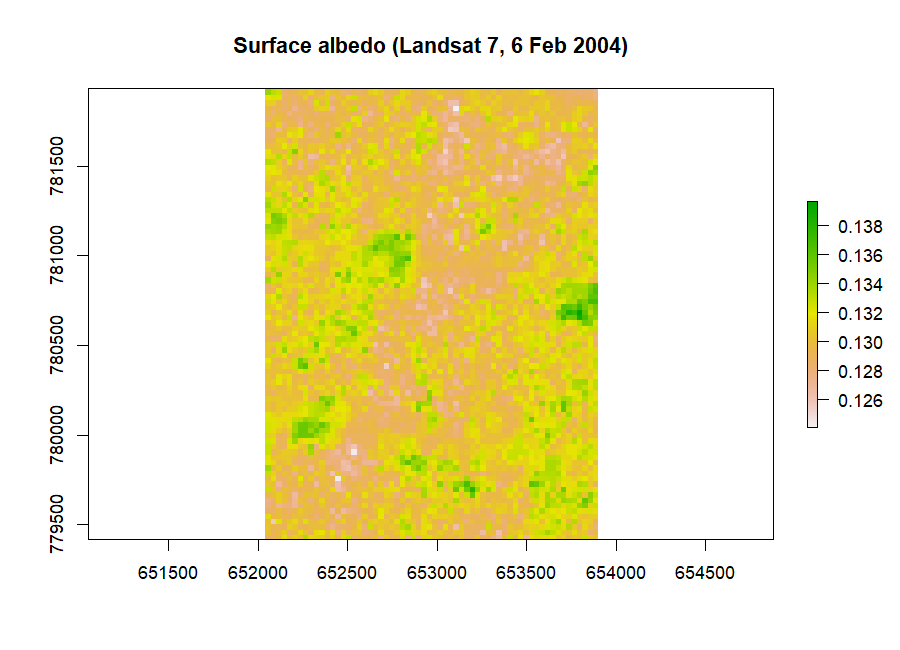
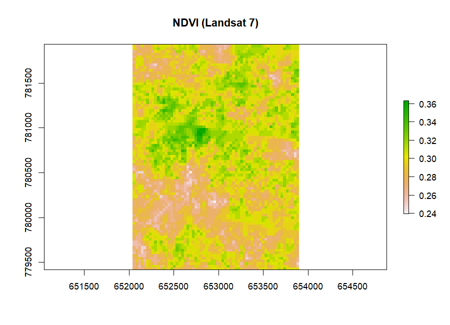
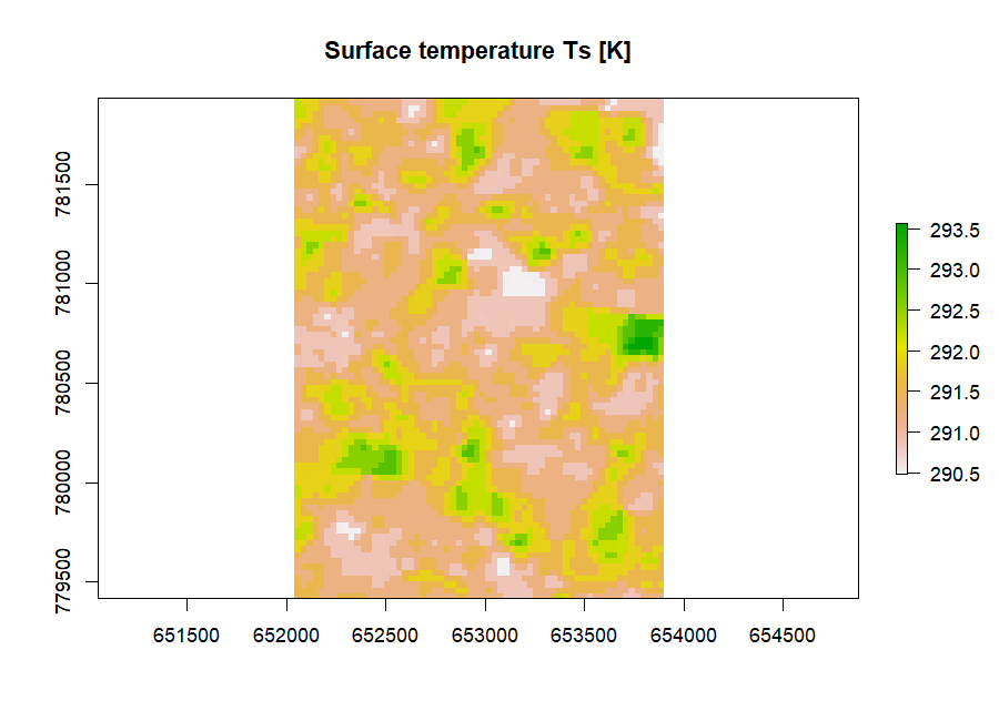
On the bundled Landsat-7 subset this returns (Figures 2–4):

Table 3: Radiometric products from landsat578 on the bundled Landsat-7 scene.

Product	min	mean	max
albedo	0.124	0.130	0.140
NDVI	0.240	0.296	0.363
SAVI	0.112	0.141	0.181
Ts [K]	290.5	291.5	293.6

Point data= at a scene folder instead and landsat578 reads the metadata and finds the Landsat-8 rescaling factors automatically. The returned object plugs straight into every model below.

$Figure 2: Surface albedo from the Landsat-7 scene (fraction of incoming shortwave reflected).$

Figure 2: Surface albedo from the Landsat-7 scene (fraction of incoming shortwave reflected).

Figure 3: NDVI — the normalised vegetation index; higher = greener, more transpiring vegetation.

Figure 4: Surface temperature Ts in kelvin, from the thermal band. Hot, dry surfaces evaporate little; cool surfaces are wet or vegetated.

12. `coldTs` / `hotTs`: the anchor pixels

SEBAL and METRIC calibrate the sensible-heat term against two anchor pixels — a cold/wet pixel (well-watered vegetation, where nearly all energy goes to ET, so H ≈ 0) and a hot/dry pixel (bare, dry soil, where LE ≈ 0, so H ≈ Rn−G). The near-linear relationship between surface temperature and H is fixed by these two ends. coldTs() and hotTs() find them automatically by k-means clustering on temperature, NDVI and albedo.

A note on the two bundled scenes. Part 2’s energy-balance demonstrations (Sections 12–17) run on the pre-processed rasters albedo.grd, Ts.grd, NDVI.grd and LAI.grd — a warmer Kumasi scene with Ts 304–313 K, supplied ready-made so the models can be shown without repeating Section 11’s preprocessing (which used a separate, cooler Landsat-7 date, Ts ≈ 291 K). That is why the temperatures jump between the two sections. Load the model inputs once:
albedo <- raster(system.file("extdata","albedo.grd", package = "sebkc"))
Ts     <- raster(system.file("extdata","Ts.grd",     package = "sebkc"))
NDVI   <- raster(system.file("extdata","NDVI.grd",   package = "sebkc"))
LAI    <- raster(system.file("extdata","LAI.grd",    package = "sebkc"))

cold <- coldTs(Ts = Ts, NDVI = NDVI, albedo = albedo, sunangle = 50,
               cluster = 7, extent = "full", seed = 1)
cold$Tscold    #> 304.89   K  (x = 259447, y = 292882)
hot  <- hotTs(Ts = Ts, NDVI = NDVI, albedo = albedo, cluster = 7,
              extent = "full", seed = 1)
hot$Tshot      #> 311.98   K  (x = 260737, y = 294412)

On the bundled Kumasi scene (Ts 304–313 K) the cold pixel sits at 304.89 K and the hot pixel at 311.98 K — a 7 K spread that anchors the H model. extent= controls the search: "full" uses the whole image, "auto" the middle portion, and "interactive" lets you digitise a polygon on the temperature map. Pass seed= for reproducible pixel selection (k-means is otherwise random). The energy-balance functions accept xyhot="auto"/xycold="auto" to run this for you.

13. `sebal`: SEBAL and METRIC

sebal() computes the full Bastiaanssen (1998) SEBAL energy balance — and, with model="METRIC", the Allen et al. (2007) METRIC variant that anchors the hot/ cold pixels to a reference ET instead of to bare extremes. It returns the whole balance as rasters:

m <- sebal(albedo = albedo, Ts = Ts, NDVI = NDVI, LAI = LAI,
           iter.max = 7, xyhot = "full", xycold = "full",
           DOY = 37, sunelev = 50.71154048, welev = 317.1, model = "SEBAL")

Table 4: SEBAL energy-balance components on the bundled Kumasi scene [W/m²].

Component	min	mean	max
`Rn` net radiation	371	419	455
`G` soil heat flux	55	69	206
`H` sensible heat	−29	179	401
`LE` latent heat (ET)	−125	171	415
`EF` evaporative fraction	0.00	0.523	1.10

How SEBAL solves for H (the hard step). Sensible heat is $H = \rho\,c_p\,dT / r_{ah}$ , where $dT$ is the near-surface air-temperature difference and $r_{ah}$ the aerodynamic resistance. Neither is known a priori, so SEBAL assumes $dT = a + b\,T_s$ is linear in surface temperature, fixes $a,b$ from the two anchor pixels ( $H\approx0$ at the cold pixel, $H\approx R_n-G$ at the hot pixel), and iterates: compute $H$ , update the atmospheric stability (Monin–Obukhov length) and $r_{ah}$ , recompute $H$ , until it converges (iter.max, default 7). Then $LE = R_n - G - H$ and $EF = LE/(R_n-G)$ .

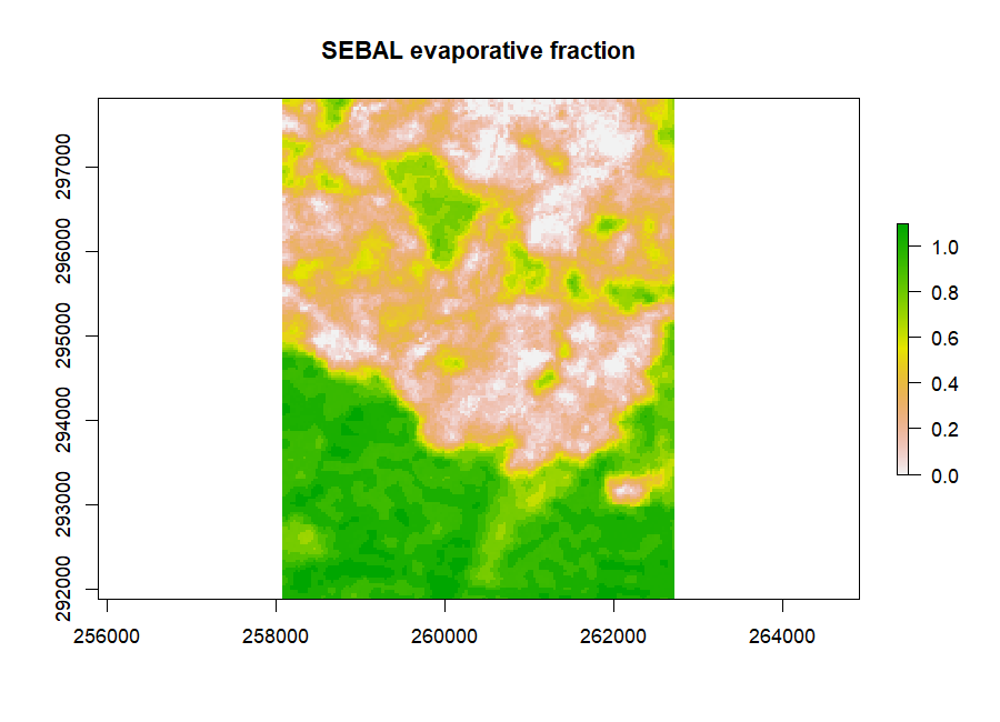
The mean EF of 0.52 says about half the available energy over the scene goes to ET; the map (Figure 5) shows the vegetated south (green, EF near 1) evaporating freely while the built-up centre of Kumasi (pink, EF near 0) does not — the urban heat-and-dryness signature, mapped. Supply Rn24= (a 24-hour net radiation, easily had from ETo) to convert EF into a daily ET map (ET24).

A handful of edge pixels report EF slightly above 1 (max 1.10) or a small negative LE (min −125 W/m²). These are not physical — they are artifacts of extrapolating the anchor-pixel calibration to the scene margins. Mask or clip the borders before using the product, and treat EF as bounded to [0, 1].

Running METRIC. METRIC is SEBAL’s operational cousin: instead of anchoring the hot/cold pixels to bare/wet extremes, it ties them to a reference ET (from a weather station), and it corrects surface temperature for terrain with a DEM and lapse rate. Switch it on with model="METRIC" and supply those extras:

metric <- sebal(albedo = albedo, Ts = Ts, NDVI = NDVI, LAI = LAI, DEM = dem,
                lapse = 0.0065, ETr = 0.35, ETr24 = 6, model = "METRIC",
                xyhot = "full", xycold = "full", DOY = 37, sunelev = 50.71,
                welev = 317.1)

where ETr is the alfalfa reference ET at overpass [mm/hr] and ETr24 its daily total. The bundled landsat8/DEM.tif supplies a DEM for a matching scene. (METRIC is not run in the offline reproduction because it needs a DEM co-registered to the input rasters and a reference-ET series; it is otherwise identical in output to SEBAL — Rn, G, H, LE, EF, plus an ETrF reference-ET fraction and ETins.)

$Figure 5: SEBAL evaporative fraction over Kumasi. Green (EF≈1) is wet, freely evaporating vegetation; pink/white (EF≈0) is the dry, built-up city core. Mean EF = 0.52.$

Figure 5: SEBAL evaporative fraction over Kumasi. Green (EF≈1) is wet, freely evaporating vegetation; pink/white (EF≈0) is the dry, built-up city core. Mean EF = 0.52.

14. The one-source family: `sebs`, `sebi`, `sseb`, `ssebi`

Four further one-source models trade SEBAL’s full iteration for different simplifications. All run on the same albedo/Ts/NDVI inputs and return an evaporative fraction; they differ in how they get there.

sebs — Su (2002) Surface Energy Balance System: a physically complete scheme that bounds EF between a theoretical dry limit and wet limit. Here mean EF = 0.275 (Figure 6).
sebi — Menenti & Choudhury (1993) Surface Energy Balance Index: uses the spread between a maximum and minimum surface temperature. Mean EF = 0.403.
sseb — Senay et al. (2011) Simplified SEB: the most economical model, scaling ET linearly between the average hot and cold pixel temperatures, ETf = (TH − Ts)/(TH − TC), and multiplying by reference ET. Mean EF = 0.466, and because it uses ETo internally it returns a daily ET24 directly (mean 1.31 mm/day).
ssebi — Roerink et al. (2000) S-SEBI: needs no weather at all — it reads the wet and dry edges straight off the albedo–temperature scatter of the image. Mean EF = 0.584.

sebs (albedo, Ts, Tmax = 31, Tmin = 28, RHmax = 84, RHmin = 63, NDVI, LAI,
      xyhot = "full", xycold = "full", DOY = 37, sunelev = 50.71, welev = 317.1)
ssebi(Ts = Ts, albedo = albedo, threshold = 0)     # weather-free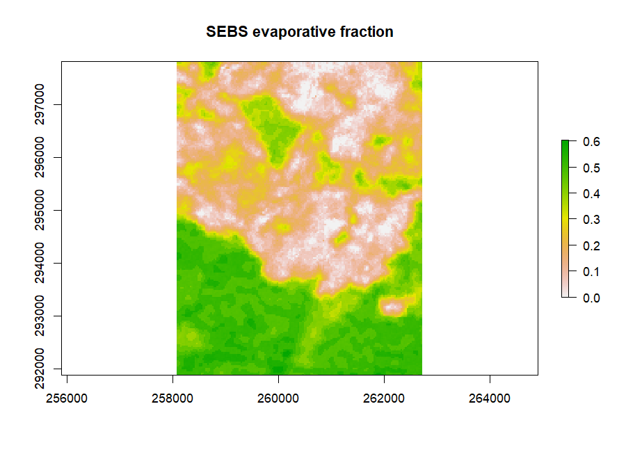

$Figure 6: SEBS evaporative fraction on the same scene (mean EF = 0.28). The spatial pattern matches SEBAL — wet south, dry city — but the level is lower, illustrating the between-model spread of Table 5.$

Figure 6: SEBS evaporative fraction on the same scene (mean EF = 0.28). The spatial pattern matches SEBAL — wet south, dry city — but the level is lower, illustrating the between-model spread of Table 5.

The SSEB shortcut (Senay et al., 2011). The simplest useful model skips the energy balance entirely and interpolates temperature between the anchors:

$ET_f = \frac{T_H - T_s}{T_H - T_C}, \qquad ET_a = ET_f \cdot ET_o$

where $T_H$ and $T_C$ are the average hot and cold pixel temperatures. A pixel as cool as the cold anchor gets $ET_f=1$ ; as hot as the hot anchor, $ET_f=0$ .

15. `tseb`: the two-source model

Where the one-source models treat each pixel as a single surface, tseb() (Norman et al., 1995; Colaizzi et al., 2012) splits it into canopy and soil, solving the energy balance separately for each and so partitioning ET into transpiration (T) and evaporation (E) — valuable for partial-cover crops. It offers a parallel network (canopy and soil resistances side by side) and a series network (coupled through a shared air temperature):

tp <- tseb(Ts, LAI, albedo = albedo, NDVI = NDVI, DOY = 37, xyhot = "full",
           xycold = "full", Tmax = 31, Tmin = 28, hc = 20, sunelev = 50,
           welev = 345, latitude = 5.6, n = 6.5, network = "parallel")
tp$ET24     # E24 (evaporation) + T24 (transpiration) also returned

On the bundled scene the parallel network gives mean ET24 = 0.54 mm/day (Figure 7) and the series network 2.27 mm/day — the two formulations differ most where cover is sparse, which is precisely the case that motivates a two-source model. series="xPT" uses the Priestley–Taylor closure, series="PM" the Penman–Monteith one.

Figure 7: TSEB (parallel) daily evapotranspiration ET24 [mm/day], partitioned internally into soil evaporation and canopy transpiration.

16. Comparing the models

Run on the same scene, the models give a spread of mean evaporative fractions — a reminder that model choice is itself a source of uncertainty:

Table 5: Mean evaporative fraction from each one-source model on the bundled Kumasi scene.

Model	Mean EF	Character
SEBS	0.275	physically bounded, conservative here
SEBI	0.403	temperature-range index
SSEB	0.466	simplest; returns ET24 directly
SEBAL	0.523	full iterative balance (reference)
S-SEBI	0.584	weather-free, image-internal edges

The models agree on the pattern — every one maps the vegetated south as wet and the city as dry — but differ on the level by nearly a factor of two. For an operational estimate, calibrate against a flux tower or a water balance if you can, and report which model you used. SSEB and S-SEBI are attractive when weather data are scarce; SEBAL/METRIC are the reference when anchor pixels and weather are good.

17. `wdi`: the water deficit index

wdi() computes the Moran et al. (1994) Water Deficit Index from surface–air temperature and vegetation, scaled between a wet edge and a dry edge:

w <- wdi(Ts = Ts, Ta = 299, NDVI = NDVI, Tsmax = 313, Tsmin = 304)
w$EF        # min 0.049  mean 0.488  max 1.000

WDI = 0 is fully watered, WDI = 1 fully stressed; the returned EF is its complement (mean 0.49 here). Supply explicit hot/cold surface temperatures (Tsmax/Tsmin) as above, or pass hotTs/coldTs objects; the "auto" edges invoke the interactive anchor routine (Section 12).

18. Coupling evaporative fraction to the FAO-56 water balance

The package’s distinctive step: feed a satellite evaporative fraction into the FAO-56 water balance (kc) instead of tabulated crop coefficients, turning a map of ET into a spatial irrigation-scheduling model. Supply the EF (from any Part-2 model) as the kc= argument and set kctype to the model:

ef  <- sebi(folder = scene, welev = 317, Tmax = 31, Tmin = 28)$EF
kc2 <- stack(ef/2, ef, ef/3)                       # EF at initial/mid/end stages
spatial <- kc(ETo = d$ETo, P = d$P, RHmin = 35, soil = "sandy loam",
              crop = "Broccoli", I = d$I, kc = kc2, Rn = 8, lengths = c(4,4,2,2))
spplot(spatial$Drend)                              # map of irrigation depth needed

Now every pixel carries its own water balance: Drend maps the irrigation depth needed to refill the root zone, Ineedxy the critically needed amount, and ETcxy the crop ET through time. Passing xydata= (longitudes/latitudes of monitoring points) with per-step precipitation interpolates sparse gauge data across the scene first. This is where Parts 1 and 2 become one model: remotely sensed actual ET driving a field-scale irrigation schedule.

PART 3 — Reference

19. Function and argument reference

Table 6: The principal sebkc functions.

Function	Purpose	Key inputs
`ETo`	24-h reference ET (FAO-56)	Tmax, Tmin, DOY, latitude (+RH, wind, sun)
`ETohr`	hourly reference ET	Tmean, RH, time, Lz, Lm, latitude
`weather`	fetch WMO/NASA weather	wmo/airport or lon/lat + dates
`kc`	crop coefficient + water balance	ETo, P, I, soil, crop (+ kc, lengths, FC, WP…)
`cal.kc`	calibrate the balance	as `kc` + measured soil water
`biomass`	crop yield	Tday, T24, Rs, latitude, plant/harvest dates
`sebkcstack`	stack/de-stripe a scene	folder
`landsat578`	bands → albedo/NDVI/Ts	data (brick or folder), welev, sensor
`coldTs`/`hotTs`	anchor pixels	Ts, NDVI, albedo, extent, seed
`sebal`	SEBAL / METRIC	albedo, Ts, NDVI, LAI, welev, DOY, sunelev, model
`sebs`/`sebi`	SEBS / SEBI EF	albedo, Ts, NDVI, Tmax, Tmin, …
`sseb`/`ssebi`	SSEB / S-SEBI	Ts, albedo (+ NDVI, weather for SSEB)
`tseb`	two-source E/T/ET	Ts, LAI, albedo, NDVI, network
`wdi`	water deficit index	Ts, Ta, NDVI, Tsmax, Tsmin

Recurring arguments: welev weather-station elevation (m); DOY day of year (or a YYYY-mm-dd date); sunelev sun elevation from the image metadata; xyhot/xycold anchor pixels ("auto", "full", coordinates, or a hotTs/coldTs object); Rn24 24-h net radiation for daily ET; folder a Landsat scene directory (bypasses manual preprocessing); iter.max sensible-heat iterations. The kc return frame’s main columns are Kc, Kcb, Ke, Ks, ETc, TAW, RAW, Drend (irrigation need), DP (deep percolation), Runoff, CN.

20. The bundled data

Everything in this manual runs on system.file("extdata", ..., package="sebkc"):

albedo.grd, Ts.grd, NDVI.grd, LAI.grd — a preprocessed Kumasi scene (Ts 304–313 K), the inputs for the energy-balance demonstrations.
landsat7_6feb2004.grd — a raw Landsat-7 band stack for landsat578.
stack/, slc/ — Landsat scene folders for the automatic (folder=) and SLC-off de-striping workflows.
landsat8/ — full Landsat-8 scenes with a DEM, for METRIC.
sys/irrigation.txt — the 12-day irrigation record used in Section 7.
kc/kumasi*.rds — Kumasi crop-coefficient time series (1960–2015 and RCP 2.6/4.5/8.5 climate scenarios to 2050) for time-series and climate-change work.

21. Reproducing the figures

Every number and figure here comes from reproduce_manual.R:

source("reproduce_manual.R")   # writes repro_output.txt and figures/*.png

It runs reference ET, the FAO-56 kc examples and water balance, Landsat preprocessing, the anchor-pixel selection, all six energy-balance models, biomass and WDI, logging each figure ok/FAIL.

22. Glossary

Reference ET (ETo) — ET of standard well-watered grass [mm/day].
Crop coefficient (Kc) — ETc/ETo; dual = Kcb (basal) + Ke (soil evaporation).
Water-stress coefficient (Ks) — reduces Kc when the root zone is depleted.
TAW / RAW — total / readily available soil water in the root zone [mm].
Net radiation (Rn), soil heat (G), sensible heat (H), latent heat (LE) — the energy-balance terms [W/m²]; Rn = G + H + LE.
Evaporative fraction (EF) — LE/(Rn−G); the share of energy going to ET.
Albedo / NDVI / Ts — surface reflectance / greenness / temperature from imagery.
Anchor (hot/cold) pixels — dry and wet reference pixels that calibrate H.
SEBAL, METRIC, SEBS, SEBI, SSEB, S-SEBI, TSEB — surface-energy-balance models.

23. Exercises

Reference ET. Compute ETo for a day with Tmax = 34, Tmin = 24, latitude 6, DOY 100, using only temperature. Then add RHmax/RHmin and sunshine and compare — how much does the estimate move?
Crop coefficient. Reproduce FAO-56 Example 32, then change fw from sprinkler to "drip"; why does Kc_adj fall?
Water balance. Run the 12-day irrigation.txt balance; on which day does the modelled available water first exceed RAW, and what does that imply for irrigation timing?
Anchor pixels. Run hotTs/coldTs on the bundled scene with seed=1 and again with seed=2; how much do Tshot/Tscold move, and what does that do to SEBAL’s EF?
Model comparison. Run sebal, sebs and ssebi on the bundled rasters and map the three EFs side by side. Where do they agree, and where most disagree?

PART 4 — Projects

This part turns the manual into coursework. Each project reruns the same method you learned in Parts 1–2 on a new scene, catchment or crop, so a student can go from raw imagery and weather to a mapped, publishable ET result by following the section references back to the worked Kumasi example. The projects suit MPhil and PhD students in geography, agronomy, irrigation engineering, hydrology and remote sensing. Assign one per student.

24. The project brief template

Every project below follows this eight-part structure. Read it once; each project then fills in its specifics.

Research question — the one- or two-sentence question the ET estimate answers.
Data source — a named, citable dataset with a working link: the satellite scene, the weather record, the boundary, and the DEM/soil if needed. Note the acquisition date and that all rasters must share one projection and extent.
Input mapping — map your data to sebkc’s inputs: a raw scene → landsat578 (with welev, sensor, sunelev, K1/K2 or Landsat-8 rescale factors from the MTL metadata); weather (Tmax, Tmin, RH, wind, DOY) → ETo/kc; crop + soil → kc (FAO-56 tables). Identify which variable plays the role Ts plays here (the thermal driver of H), and which plays ETo (the climatic demand).
Step-by-step, cross-referenced to the manual: preprocess (Section 11), pick anchor pixels (Section 12), run a model (Sections 13–15), upscale to daily ET with Rn24 from ETo (Section 13), and — if scheduling irrigation — couple EF into kc (Section 18).
Expected output shape — an EF map bounded to [0, 1] (wet vegetation high, dry/bare/urban low), an ET24 map in mm/day of plausible magnitude (a few mm/day for cropland), and a kc water-balance table.
Interpretation checklist — Is the EF pattern physically sensible against land cover? Do the hot/cold anchor pixels sit on genuinely dry and wet surfaces? Does ET24 fall in a credible range? For a catchment, does the water balance (P − ET − runoff) close?
Validation / sensitivity extension — compare against a flux tower or lysimeter where available (FLUXNET https://fluxnet.org), or against a MODIS ET product (MOD16); test anchor-pixel sensitivity by re-running with different seed= or extent= (Section 12).
Deliverable — a short paper (Introduction / Data / Method / Results / Discussion) modelled on this manual’s own prose, of a standard that could be submitted to a journal.

Common data portals used below: Landsat / SRTM DEM — USGS EarthExplorer https://earthexplorer.usgs.gov; Sentinel-2/3 — Copernicus Data Space https://dataspace.copernicus.eu; weather & solar — NASA POWER https://power.larc.nasa.gov; rainfall — CHIRPS https://www.chc.ucsb.edu/data/chirps; MODIS ET (MOD16) — LP DAAC https://lpdaac.usgs.gov; soil — SoilGrids https://soilgrids.org or FAO HWSD https://www.fao.org/soils-portal; boundaries — GADM https://gadm.org; cloud processing — Google Earth Engine https://earthengine.google.com.

25. Agriculture and irrigation projects

Project 1 — Irrigation scheduling for a scheme. Question: how much water does an irrigation scheme need, field by field, this week? Data: a Landsat scene over the scheme (EarthExplorer) + a nearby weather record (NASA POWER) + scheme field boundaries (Ghana Irrigation Development Authority, via the Ministry of Food and Agriculture https://mofa.gov.gh). Method: landsat578 → SEBAL/SSEB EF (Sections 11–14) → couple EF into kc (Section 18) to map Drend (the irrigation depth needed). Deliverable: a field-level irrigation schedule with an irrigation-need map.

Project 2 — Crop water-requirement mapping for a district. Question: what is the seasonal crop ET (ETc) across a farming district? Data: multi-date Landsat + FAO-56 crop and soil parameters + district boundary (GADM). Method: kc single/dual coefficient driven by station ETo (Sections 4, 7), mapped per land parcel. Deliverable: a seasonal ETc and water-demand paper.

Project 3 — Water productivity and deficit irrigation. Question: how much crop yield is produced per unit of water evapotranspired? Data: a Landsat ET map + a yield survey or biomass estimate. Method: SEBAL ET24 (Section 13) against biomass yield (Section 9); map ET, yield and their ratio. Deliverable: a water-productivity study identifying where water is used efficiently.

Project 4 — Rice vs maize water use. Question: how do the seasonal ET and Kc curves of two crops compare? Data: two fields of known crop + a season of Landsat + weather. Method: dual-kc curves (Section 7) and satellite EF (Section 14) per field. Deliverable: a comparative crop-water-use paper.

26. Hydrology and water-resources projects

Project 5 — Catchment actual ET for a water balance. Question: how much water leaves a catchment as ET, and does the basin balance close? Data: Landsat/MODIS over the catchment + CHIRPS rainfall + a DEM (SRTM) + catchment boundary (HydroSHEDS). Method: SEBAL or SSEB ET24 aggregated to the catchment (Sections 13–14); compare P − ET to observed runoff. Deliverable: a basin water-balance paper.

Project 6 — Open-water and wetland evaporation. Question: how much water evaporates from a reservoir or wetland? Data: Landsat thermal + a water mask + weather. Method: EF/ET24 restricted to the water body, cross-checked against a pan or energy-budget estimate. Deliverable: a reservoir-loss study for water-resource planning.

Project 7 — Groundwater-recharge screening. Question: where might recharge occur (rainfall minus ET minus runoff > 0)? Data: CHIRPS rainfall + Landsat ET + a runoff estimate. Method: map the residual P − ET − runoff. Deliverable: a recharge-potential map and note.

27. Remote-sensing and land-surface projects

Project 8 — ET by land-cover class. Question: how does ET differ across land-cover types? Data: a Landsat ET map + a land-cover classification (or ESA WorldCover). Method: zonal statistics of ET24/EF (Section 13) by class. Deliverable: an ET-signature paper for the region’s land covers.

Project 9 — Multi-model ET intercomparison. Question: how far do the SEB models disagree on one scene, and why? Data: one Landsat scene. Method: run sebal, sebs, sebi, sseb, ssebi and tseb (Sections 13–15) and compare maps and means (Section 16). Spatial: validate against a flux tower if available. Deliverable: a model-intercomparison paper — recommended as an early, self-contained project.

Project 10 — Landsat SEBAL vs MODIS MOD16. Question: how does a sebkc ET map compare with the operational MODIS product? Data: a Landsat scene + the matching MOD16 tile (LP DAAC). Method: SEBAL ET24 (Section 13) resampled to MODIS and differenced. Deliverable: a product-comparison paper.

Project 11 — Seasonal ET dynamics. Question: how does ET evolve through a growing season? Data: a time series of cloud-free Landsat/Sentinel-2 dates over a field. Method: EF/ET24 per date (Sections 11–14); plot the ET trajectory. Deliverable: a seasonal-ET-dynamics paper.

28. Climate and environment projects

Project 12 — Climate-change reference ET and crop water demand. Question: how will crop water demand shift under future climate? Data: the bundled Kumasi RCP crop-coefficient series (kc/kumasircp*2016_2050.rds) or downscaled WorldClim/CMIP projections + baseline ETo. Method: recompute ETo and the kc water balance under RCP 2.6/4.5/8.5 (Sections 4, 7); compare irrigation need. Deliverable: a climate-change irrigation-demand paper — a PhD-level extension.

Project 13 — Urban heat and evapotranspiration. Question: how much lower is ET over the built city than the surrounding countryside? Data: a Landsat scene over a city (the bundled Kumasi scene is a ready example). Method: EF/Ts contrast between urban and rural pixels (Sections 12–13). Deliverable: an urban-heat / green-cooling paper.

Project 14 — Agricultural drought monitoring with the WDI. Question: which fields are under water stress right now? Data: a recent Landsat scene + air temperature. Method: wdi (Section 17) with explicit hot/cold surface temperatures; map the deficit index over time. Deliverable: a drought-monitoring bulletin.

29. Methods project

Project 15 — Anchor-pixel calibration sensitivity. Question: how much does the automatic anchor-pixel selection move the ET estimate? Data: one Landsat scene. Method: run sebal with xy="auto"/"full" and with interactively digitised anchors, and across several seed= values (Sections 12–13); quantify the EF spread. Spatial: Not applicable — the point is calibration robustness, not spatial pattern. Deliverable: a methods note on calibration uncertainty in one-source SEB models.

(Fifteen projects. If fewer are needed, trim from Agriculture or Remote-sensing where routes overlap; keep Project 9 — the model intercomparison — as it exercises the whole Part 2 toolkit at once.)

How to cite this manual

If you use sebkc or this manual in published work, please cite the package:

Owusu, G. (2026). sebkc: Surface Energy Balance and Crop Coefficient Evapotranspiration Estimation. R package version 1.0-7. https://doi.org/10.32614/CRAN.package.sebkc

@Manual{sebkc,
  title  = {sebkc: Surface Energy Balance and Crop Coefficient
            Evapotranspiration Estimation},
  author = {George Owusu},
  year   = {2026},
  note   = {R package version 1.0-7},
  doi    = {10.32614/CRAN.package.sebkc}
}

And this manual:

Owusu, G. (2026). sebkc: A manual to surface energy balance and crop-coefficient evapotranspiration in R (Version 1.0-7). Department of Geography and Resource Development, University of Ghana.

The methods rest on the FAO-56 paper (Allen et al., 1998), SEBAL (Bastiaanssen et al., 1998), METRIC (Allen et al., 2007) and the other model references below; cite the relevant original alongside the package.

References

Allen, R. G., Pereira, L. S., Raes, D., & Smith, M. (1998). Crop Evapotranspiration — Guidelines for Computing Crop Water Requirements. FAO Irrigation and Drainage Paper 56. Rome: FAO.
Allen, R., Tasumi, M., & Trezza, R. (2007). Satellite-based energy balance for mapping evapotranspiration with internalized calibration (METRIC) — Model. Journal of Irrigation and Drainage Engineering, 133(4), 380–394.
Bastiaanssen, W. G. M., Menenti, M., Feddes, R. A., & Holtslag, A. A. M. (1998). A remote sensing surface energy balance algorithm for land (SEBAL), part 1: formulation. Journal of Hydrology, 212–213, 198–212.
Chander, G., Markham, B. L., & Helder, D. L. (2009). Summary of current radiometric calibration coefficients for Landsat sensors. Remote Sensing of Environment, 113(5), 893–903.
Menenti, M., & Choudhury, B. (1993). Parameterization of land surface evaporation by means of location-dependent potential evaporation and surface temperature range (SEBI). IAHS Publication, 212.
Moran, M. S., Clarke, T. R., Inoue, Y., & Vidal, A. (1994). Estimating crop water deficit using the relation between surface–air temperature and spectral vegetation index (WDI). Remote Sensing of Environment, 49(3), 246–263.
Norman, J. M., Kustas, W. P., & Humes, K. S. (1995). A two-source approach for estimating soil and vegetation energy fluxes (TSEB). Agricultural and Forest Meteorology, 77, 263–293.
Colaizzi, P. D., et al. (2012). Two-source energy balance model estimates of evapotranspiration using component and composite surface temperatures. Advances in Water Resources.
Roerink, G. J., Su, Z., & Menenti, M. (2000). S-SEBI: a simple remote sensing algorithm to estimate the surface energy balance. Physics and Chemistry of the Earth (B), 25(2), 147–157.
Senay, G. B., Budde, M. E., & Verdin, J. P. (2011). Enhancing the Simplified Surface Energy Balance (SSEB) approach. Agricultural Water Management, 98(4), 606–618.
Su, Z. (2002). The Surface Energy Balance System (SEBS) for estimation of turbulent heat fluxes. Hydrology and Earth System Sciences, 6(1), 85–100.
Owusu, G. (2026). sebkc: Surface Energy Balance and Crop Coefficient Evapotranspiration Estimation. R package version 1.0-7. https://doi.org/10.32614/CRAN.package.sebkc

sebkc — surface energy balance and crop-coefficient evapotranspiration for R. This manual and all its numbers were produced by running the package on its bundled Kumasi Landsat data and FAO-56 examples (R 4.6.0, sebkc 1.0-7).

Contents